Inside BraiNN: Anatomy, Dynamics, Fields, and EEG in One Workflow

by IT’IS Foundation
The whole-brain scale. Scalp EEG mainly reflects the summed postsynaptic activity of large neuronal populations, rather than individual spikes. Neural mass models describe activity at this scale through mean membrane potentials and firing rates, with each population evolving according to its local dynamics and the input it receives from the network. The same class of model underlies the Virtual Epileptic Patient, which runs a neural mass model of seizure dynamics in The Virtual Brain [1, 2]. In a retrospective study, its estimates agreed with the clinically defined epileptogenic networks, most closely in patients who became seizure-free after resection [3].

BraiNN supports two resolutions. In a region-level network, a single neural mass node represents each anatomical region. In a cortical-surface network, every vertex of a (potentially personalized) cortical mesh carries a complete node; sparse, geodesic-distance-dependent connectivity describes local interactions, and long-range interactions are inherited from the region-level structural connectivity. This preserves spatial detail within regions while retaining anatomically meaningful connections between them.

The neural mass model. Each node is a Jansen-Rit model of a cortical column [6] comprising pyramidal projection neurons and excitatory and inhibitory interneuron populations (the solver library also supports other model variants). The model's state variables represent mean membrane potentials, and a sigmoid function translates the membrane potentials into firing rates. The node's output – i.e., the difference between the excitatory and inhibitory postsynaptic potentials of the pyramidal population – is passed to other nodes (see below) and, after conversion to an equivalent current dipole, serves to generate virtual EEG signals.

The model uses a standard parameterization from the literature [6], and key parameters are exposed to the user: the excitatory and inhibitory synaptic gains set the balance of excitation and inhibition within each column; the global coupling strength scales long-range input; the local surface coupling strength governs interactions between neighboring surface nodes; and — for the stochastic differential equation variant — a noise scaling factor multiplies a literature-based noise structure [10]. Varying these parameters lets researchers explore local rhythms, synchronization across regions, and the sensitivity of the simulated signal to the noise level.

Connectivity and delays. Long-range input to each node is a weighted sum of the delayed outputs of the other regions, which in surface networks are the mean pyramidal outputs of the surface nodes assigned to each region. The weights come from structural connectivity derived from diffusion tractography, and the delays from tract lengths and an assumed conduction speed; a global coupling strength scales the weighted sum.

From activity to EEG. Simulated cortical activity contributes to scalp potentials according to weightings in a lead-field matrix: each cortical source is represented as an equivalent current dipole normal to the local cortical surface, and the matrix maps the dipole moments to electrode voltages. Sim4Life computes the lead field through Plonsey's reciprocity theorem [11]: a low-frequency electromagnetic simulation applies a unit current between each EEG electrode and a common reference, and the normal component of the resulting field at each cortical vertex gives that electrode's lead-field weight. The stimulation field and EEG lead fields use the same head model and electromagnetic physics, so both calculations share anatomy, tissue properties, and coordinate frame.

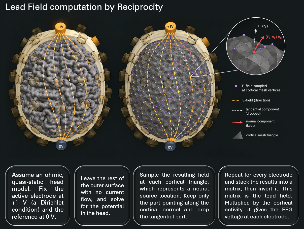Lead fields by reciprocity: A unit current between an electrode and the reference produces an electric field in the head model. Its normal component on the cortical surface provides the weights for projecting simulated cortical activity to that electrode. The same head model is used to compute the stimulation field.

From field to input. A stimulation field enters the network through a λE∥ coupling term [7 – 9]: the field component parallel to the modeled cortical columns (i.e., normal to the cortical surface) is scaled by a population-specific factor λ. The result is added to each population's mean membrane potential as a field-induced polarization. In V10.0, this field-induced contribution is constant in time; support for time-varying stimulation is planned for a future release. How an electric field translates into the behavior of a whole population of neurons is still an open research question; the coupling model therefore remains a subject for further investigation.

The numerical engine. BraiNN is implemented in JAX, with the integration loop, network coupling, stochastic noise, and monitoring compiled together, so that the same model definition runs on CPUs, GPUs, or tensor processing units. Joint arrays vectorize operations over nodes and over batches of parameter sets, initial conditions, or noise realizations.

On a GPU, BraiNN runs whole-brain simulations orders of magnitude faster than commonly used CPU-based simulators. In the preprint's benchmarks [5], measured on an NVIDIA RTX 3090 GPU against The Virtual Brain on a 32-core AMD Ryzen Threadripper 3970X CPU, a region-level network of 68 regions ran about 35× faster, and a cortical-surface network of 4.4k nodes about 90× faster. Runtime changed little with network size up to 250 regions, and adding conduction delays or batching runs increased it only slightly, so a batch of parameter sets costs little more than a single simulation. Previously intractable parameter sweeps, response-surface exploration, and sensitivity analyses therefore become practical, as do the fitting procedures described below (Outlook).

A deterministic/stochastic switch selects the solver family: deterministic runs can use forward Euler, Heun, classical fourth-order Runge-Kutta, or the adaptive Tsit5 and Dormand-Prince time-integration methods, while stochastic runs handle additive noise with Euler-Maruyama, stochastic Heun, or higher-order splitting Runge-Kutta methods. Selecting stochastic mode also exposes the noise scaling factor.

Monitoring is decoupled from the time-discretization step, so regional firing rates, cortical source activity, and electrode voltages can be recorded at a lower rate without altering the numerical integration. Simulations use 32-bit precision by default, with a 64-bit option for verification and sensitivity studies.

What V10.0 delivers. V10.0 provides the forward pipeline from structure and dynamics through stimulus coupling to EEG projection, together with a predefined model set, adjustable parameters, and a direct link to Sim4Life's field solvers.

Outlook. Two extensions, both addressing personalization, are in preparation. Image-based model generation builds the head model, cortical mesh, structural connectivity, and lead fields from a subject's T1-weighted and diffusion magnetic resonance imaging (MRI) scan, so that the stimulation field, network, and simulated EEG all reflect the subject's anatomy. EEG-based parameter fitting uses Bayesian optimization to adjust the neural mass parameters until the simulated EEG best reproduces the subject's recordings [5]. Fitting in this way requires a large number of forward simulations, which is where BraiNN's speed matters most. Together, these extensions bring the personalization demonstrated in epileptic focus mapping [3] to brain stimulation.

BraiNN is a research tool for studying whole-brain dynamics and stimulation, and its results should be interpreted in light of the modeling assumptions described above. The preprint [5] describes the methods in detail. Sim4Life V10.0 integrates this engine with Virtual Population and image-based head models, field simulators, visualization, and analysis. Anatomy extraction, field calculations, network modeling, and virtual EEG generation thus stay within a single Sim4Life project, without the compatibility and versioning issues that arise with multiple tools.

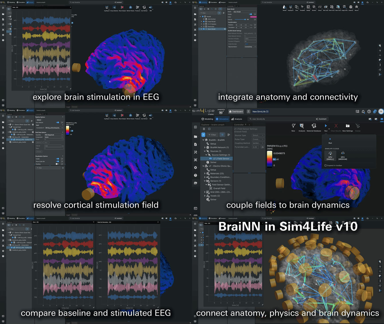BraiNN: From Stimulation Field to Simulated EEG.

References
[1] Sanz Leon P, et al. The Virtual Brain: A simulator of primate brain network dynamics. Front Neuroinform. 2013;7:10. https://doi.org/10.3389/fninf.2013.00010
[2] Jirsa VK, et al. On the nature of seizure dynamics. Brain. 2014;137(8):2210-2230. https://doi.org/10.1093/brain/awu133
[3] Wang HE, et al. Delineating epileptogenic networks using brain imaging data and personalized modeling in drug-resistant epilepsy. Sci Transl Med. 2023;15(680):eabp8982. https://doi.org/10.1126/scitranslmed.abp8982
[4] Wang HE, et al. Virtual brain twins for stimulation in epilepsy. Nat Comput Sci. 2025;5(9):754-768. https://doi.org/10.1038/s43588-025-00841-6
[5] Fasse A, et al. BraiNN: A modern simulator for clinically feasible personalized whole-brain network modeling. bioRxiv. 2026. https://doi.org/10.64898/2026.07.08.737156
[6] Jansen BH, et al. Electroencephalogram and visual evoked potential generation in a mathematical model of coupled cortical columns. Biol Cybern. 1995;73(4):357-366. https://doi.org/10.1007/BF00199471
[7] Molaee-Ardekani B, et al. Effects of transcranial direct current stimulation (tDCS) on cortical activity: a computational modeling study. Brain Stimul. 2013;6(1):25-39. https://doi.org/10.1016/j.brs.2011.12.006
[8] Merlet I, et al. From oscillatory transcranial current stimulation to scalp EEG changes: A biophysical and physiological modeling study. PLoS ONE. 2013;8(2):e57330. https://doi.org/10.1371/journal.pone.0057330
[9] Kunze T, et al. Transcranial direct current stimulation changes resting state functional connectivity: A large-scale brain network modeling study. NeuroImage. 2016;140:174-187. https://doi.org/10.1016/j.neuroimage.2016.02.015
[10] Ableidinger M, et al. A stochastic version of the Jansen and Rit neural mass model: Analysis and numerics. J Math Neurosci. 2017;7:8. https://doi.org/10.1186/s13408-017-0046-4
[11] Plonsey R. Reciprocity applied to volume conductors and the ECG. IEEE Trans Biomed Electron. 1963;10(1):9-12. https://doi.org/10.1109/TBMEL.1963.4322775